機械学習におけるデータ分割手法まとめ

機械学習において，持っているデータ全てを学習させてしまうと，そのデータの傾向に依存したバイアスがかかり，過学習に陥ることによって，モデルにおける未知のデータに対する推論性能（汎化性能）が損なわれる恐れがあります．
これの対策の一つとして，データ全てを学習させるのではなく，学習用データと検証用データに分けておくことで，モデルの汎化性能を測定することができます．
また，検証用データの推論結果と正解データの差（エラー）を取り，これを最小化することで，モデルにおける汎化性能を向上させることも可能です．

Python における代表的な機械学習ライブラリの scikit-learn では，データ分割に用いることのできる便利なクラスや関数はいくつかあるのですが，挙動が自分の中で不明確なものもあり，使いこなせていない感覚があったのでここをクリアにすべくまとめました．
もちろん，公式サイト (https://scikit-learn.org/stable/auto_examples/model_selection/plot_cv_indices.html#sphx-glr-auto-examples-model-selection-plot-cv-indices-py) においても網羅的で素晴らしいドキュメントが掲載されているのですが，個人的に不明な点があったため，もう一歩納得行くように検討を加えてみます．

以下掲載のコードは，次の github にも載せています．

PythonCourse/crossval.ipynb at main · KazutoMakino/PythonCourse

Python Course. Contribute to KazutoMakino/PythonCourse development by creating an account on GitHub.

scikit-learn に含まれるデータ分割のクラス／関数一覧と特徴
データとその可視化用の処理の準備
データ分割の実装例と説明

scikit-learn に含まれるデータ分割のクラス／関数一覧と特徴

データ分割手法は大きく二つに分けられます．

ホールドアウト検証
- シンプルに学習用と検証用でデータを2つに分け，検証用データは一度も学習に用いることはありません
- データ数が十分多い時だったり，学習の処理が重い場合に用います．
- データの割合として，学習用：検証用＝ 9：1 とか 8：2 にする場合が多い印象です
交差検証 (CV; Cross-Validation)
- 学習用／検証用データを複数パターン用意して学習できるので，手持ちのデータをフル活用できたり，データ分割の方法によっては汎化性能を持たせることができます．
- データを分割した個数分，計算負荷／時間は増加します．
- こちらの記事 (https://datachemeng.com/post-3484/) によるとデータ分割の割合はおおよそ以下の通りとのことで，参考までに掲載いたします．
  - 1000 サンプル以上 : 2 分割 cross-validation
  - 1000 ~ 100 : 5 分割
  - 100 ~ 30 : 10 分割 cross-validation
  - 30 以下 : leave-one-out

ホールドアウト検証，交差検証の一覧と使いどころは以下です．

クラス／関数	説明
sklearn.model_selection.check_cv	cross-validator オブジェクト（KFold など）について確認ができます．一応関数は用意されていますが，使ったことはありません．
sklearn.model_selection.train_test_split	学習用データと検証用データを2つに分けます（ホールド・アウト検証）．元データの量がかなり多いとき（どれくらいとは言っていない）や，学習の処理が重くて以下の交差検証するのが厳しい場合に用います．データの割合として，学習用：検証用＝ 9：1 とか 8：2 にする場合が多い印象です．
sklearn.model_selection.KFold	データを指定した K 個に等分し，1 つを検証用，それ以外の K-1 個を学習に用います．各 fold における検証用データに重複はさせないようにします．学習用／検証用データに偏りが出る可能性があるので他の分割手法を用いることが多いと思いますが，元データと実装後のデータがどれを取っても偏りがなさそうであれば，KFold を用いても良いでしょう．
sklearn.model_selection.ShuffleSplit	train_test.split(shuffle=True, stratify=None) を複数回作用させるような学習用／検証用データのインデックスを返すオブジェクトを生成します．各 fold における検証用データは重複します．検証用データが重複したり，ある学習用データが学習されなかったりするので，あまり使われないイメージです．
sklearn.model_selection.StratifiedKFold	データを指定した K 個に等分し，1 つを検証用，それ以外の K-1 個を学習に用います．データ分割の際には，メソッド split の引数 y にてラベルやグループを指定することにより，全種類のラベルも均等に分割されます．各 fold における検証用データは重複させないようにします．学習／検証に用いることができる手元にあるデータと推論対象のデータが同等のものであれば，有益なデータ分割手法です．推論対象のデータが学習するデータとは異質である場合は過学習気味になり，汎化性能が損なわれる可能性があります．
sklearn.model_selection.StratifiedShuffleSplit	train_test.split(shuffle=True, stratify=y) を複数回作用させるような学習用／検証用データのインデックスを返すオブジェクトを生成します．各 fold における検証用データは重複します．検証用データが重複したり，ある学習用データが学習されなかったりするので，あまり使われないイメージです．
sklearn.model_selection.GroupKFold	データを指定した K 個に分割し，1 つを検証用，それ以外の K-1 個を学習に用います．データ分割の際には，メソッド split の引数 groups にて指定したグループによって，分割するインデックスを制御します．各 fold における検証用データに重複させないようにします．グループを分けて学習することで汎化性能を得やすく，手元にあるデータと，モデル構築後の推論対象データの差がある場合でも上手く機能します．
sklearn.model_selection.GroupShuffleSplit	GroupKFold のデータ分割で，各 fold 間におけるグループの重複を許したデータ分割手法．検証用データが重複したり，ある学習用データが学習されなかったりするので，あまり使われないイメージです．
sklearn.model_selection.StratifiedGroupKFold	データを指定した K 個に分割し，1 つを検証用，それ以外の K-1 個を学習に用います．データ分割は，メソッド split の引数 y にて指定したラベル，groups にて指定したグループを用いて，グループのまとまりを使ってラベルを K 個に均等に分けるように作用します．イメージとしては，名前の通り StratifiedKFold と GroupKFold が合体したものです．各 fold における検証用データのグループは重複しません． GroupKFold に加えて，ラベルの分割についても考慮したい場合はこちらを用います．
sklearn.model_selection.RepeatedKFold	KFold を n_repeats で指定した回数分行います．リピートされる各 fold 間では検証用データの重複はありませんが，各リピート間では検証用データの重複は発生します．実装されているコードをあまり見たことはありませんが，データ数が少ないときに使えるかもしれません．
sklearn.model_selection.RepeatedStratifiedKFold	StratifiedKFold を n_repeats で指定した回数分行います．リピートされる各 fold 間では検証用データの重複はありませんが，各リピート間では検証用データの重複は発生します．実装されているコードをあまり見たことはありませんが，データ数が少ないときに使えるかもしれません．
sklearn.model_selection.LeaveOneOut	一つだけを検証用データ，その他は学習用データとして分割します．データ数が極端に少ないときに用います．
sklearn.model_selection.LeavePOut	引数 p で指定した個数を検証用データ，その他を学習用データとして分割します．検証用データが複数の場合は，検証用データの組み合わせが各 fold にて重複しないように，網羅的に fold が設定されます．例えば，データ数が m 個，引数 p を n 個と設定すると，総 fold 数は数学の組み合わせの記号 C を用いて，mCn = m(m-1) / (n(n-1)) 個生成されます．データ数が極端に少ないときに用います．
sklearn.model_selection.LeaveOneGroupOut	1 つのグループを検証用データとし，それ以外を学習用データとして分割します．グループが大まかに分かれている場合はこちらを用いることがあるかもしれません．
sklearn.model_selection.LeavePGroupsOut	引数 n_groups で指定したグループ数を検証用データ，その他を学習用データとして分割します．検証用データが複数の場合は，検証用データの組み合わせが各 fold にて重複しないように，網羅的に fold が設定されます．例えば，グループ数が m 個，引数 n_groups を n 個と設定すると，総 fold 数は数学の組み合わせの記号 C を用いて，mCn = m(m-1) / (n(n-1)) 個生成されます．グループが大まかに分かれている場合はこちらを用いることがあるかもしれません．
sklearn.model_selection.PredefinedSplit	引数 test_fold に指定した fold でデータを分割します．用意されている実装でなく，各 fold をカスタマイズしたい場合に用います．
sklearn.model_selection.TimeSeriesSplit	時系列データを考慮したデータ分割手法で，検証用データを K 等分し，残りの検証用データよりも前のデータを学習用データとして用います．したがって，index=0 から始まるような検証用データにおける学習用データは取れないので，検証用データは K-1 個になります．引数 n_splits では，この K-1 を指定します．時系列を考慮しなければならないデータの交差検証ではこちらを用います．

データ分割のクラス／関数一覧

上表の KFold 以下の交差検証クラスにおいては split というメソッドを適用させ，各 fold における学習用データと検証用データを割り振ります．
クラスによっては無い引数もありますが，split の引数は，X: 説明変数，y: 目的変数，groups: グループ　の3種類です．

では，上記をそれぞれ sklearn.model_selection を用いて実装し，データ分割について可視化していきますが，まずはその前に，データと可視化用の処理について準備します．

データとその可視化用の処理の準備

対象のデータセットとしては，フリーで有名なアヤメ（花）の品種分類データセットの “iris dataset” (https://archive.ics.uci.edu/ml/datasets/Iris) を用います．
以下のように，全データを一つの pandas.DataFrame に保存しておきます．
pandas.DataFrame にするならば，seaborn.load_dataset(“iris”) にてデータ取得するのがもっとも簡単な書き方だと思います．

from pathlib import Path

import numpy as np
import pandas as pd
import matplotlib.pyplot as plt
import seaborn as sns
from sklearn.preprocessing import LabelEncoder
sns.set()

iris = sns.load_dataset(name="iris")
print(iris)

#      sepal_length  sepal_width  petal_length  petal_width    species
# 0             5.1          3.5           1.4          0.2     setosa
# 1             4.9          3.0           1.4          0.2     setosa
# 2             4.7          3.2           1.3          0.2     setosa
# 3             4.6          3.1           1.5          0.2     setosa
# 4             5.0          3.6           1.4          0.2     setosa
# ..            ...          ...           ...          ...        ...
# 145           6.7          3.0           5.2          2.3  virginica
# 146           6.3          2.5           5.0          1.9  virginica
# 147           6.5          3.0           5.2          2.0  virginica
# 148           6.2          3.4           5.4          2.3  virginica
# 149           5.9          3.0           5.1          1.8  virginica
# 
# [150 rows x 5 columns]

データは 150 行あるのですが少し多いので，以下の通りランダムに 100 行分のデータを抜き取ります．
後ほど可視化する際に見やすいように，species で昇順に並び替えた後，行番号を振り直しています．

df = iris.sample(n=100, random_state=42)
df.sort_values(by="species", inplace=True)
df.reset_index(drop=True, inplace=True)

ここで，後ほどラベルでないグループでデータを分けることもある都合により，「調査した地域」という意味合いで “area” という名称でカラムを以下のように追加します．
※　このグループは便宜的に勝手に付け加えたものです

df["area"] = (
    ["A"] * 50
    + ["B"] * 20
    + ["C"] * 15
    + ["D"] * 10
    + ["E"] * 5
)
print(df)
#     sepal_length  sepal_width  petal_length  petal_width    species area
# 0            5.2          3.5           1.5          0.2     setosa    A
# 1            4.9          3.1           1.5          0.2     setosa    A
# 2            5.0          3.4           1.6          0.4     setosa    A
# 3            5.0          3.2           1.2          0.2     setosa    A
# 4            5.1          3.8           1.9          0.4     setosa    A
# ..           ...          ...           ...          ...        ...  ...
# 95           6.3          2.7           4.9          1.8  virginica    E
# 96           7.7          3.8           6.7          2.2  virginica    E
# 97           5.7          2.5           5.0          2.0  virginica    E
# 98           5.8          2.7           5.1          1.9  virginica    E
# 99           7.2          3.2           6.0          1.8  virginica    E
# 
# [100 rows x 6 columns]

# features / objectives
x = df[[v for v in df.columns if v!="species"]]
y = df["species"]
group = df["area"]
print(f"x.shape={x.shape}, y.shape={y.shape}, group.shape={group.shape}")
# x.shape=(100, 5), y.shape=(100,), group.shape=(100,)

print(y.value_counts())
# setosa        37
# versicolor    32
# virginica     31
# Name: species, dtype: int64

ここで，後ほど可視化に用いるためのクラスを定義しておきます．

class FoldsPlotter:
    """ Create a sample plot for indices of a cross-validation object.

    ref:
    - https://scikit-learn.org/stable/auto_examples/model_selection/plot_cv_indices.html
    """
    def __init__(
        self, x: pd.DataFrame,
        y: pd.Series,
        group: pd.Series,
        ylabel: str = "Fold indices",
        lw: int = 10,
    ) -> None:
        self.x = x
        self.y = y
        self.group = group

        # set encoder and transformed data
        enc = LabelEncoder()
        self.enc_y = enc.fit_transform(y)
        self.enc_group = enc.fit_transform(group)

        # line width
        self.lw = lw

        # plot y-axis label
        self.ylabel = ylabel

        # set save dir
        self.save_dir = Path("./out")
        None if self.save_dir.exists() else self.save_dir.mkdir()

        # init
        self.fold_num = 0
        fig = plt.figure(figsize=(8, 4), facecolor="white")
        self.ax = fig.add_subplot()

    def __del__(self) -> None:
        pass

    def get_legends(
        self,
        label_names: tuple,
        cmap_name: str = "coolwarm",
        bbox_to_anchor: tuple = (1, 1),
        loc: str = "best",
        ncol: int = 5,
        leg_title: str = "title",
    ) -> None:
        # init
        handles = []
        labels = []

        # get legend
        for i, label in enumerate(label_names):
            if len(label_names) == 1:
                color_idx = 0
            else:
                color_idx = i / (len(label_names) - 1)
            color = plt.get_cmap(cmap_name)(color_idx)
            p, = self.ax.plot([-10, -11], [-10, -10], label=label, color=color)
            handles.append(p)
            labels.append(p.get_label())
        legends = self.ax.legend(
            handles=handles,
            labels=labels,
            bbox_to_anchor=bbox_to_anchor,
            loc=loc,
            ncol=ncol,
            title=leg_title,
        )
        plt.gca().add_artist(legends)

    def add_plot(
        self,
        train_idx: np.ndarray = None,
        test_idx: np.ndarray = None,
        cmap="cool",
    ) -> None:
        if (train_idx is None) or (test_idx is None):
            return
        # fill in indices with the training / test groups
        indices = np.array([np.nan] * len(self.x))
        indices[train_idx] = 0
        indices[test_idx] = 1

        # scatter plot
        self.ax.scatter(
            x=range(len(indices)),
            y=[self.fold_num + 0.5] * len(indices),
            c=indices,
            marker="_",
            lw=self.lw,
            cmap=cmap,
        )

        # get legend
        if self.fold_num == 0:
            self.get_legends(
                label_names=("train", "test"),
                cmap_name=cmap,
                bbox_to_anchor=(1, 1),
                loc="lower right",
                leg_title="train / test",
            )

        # increment
        self.fold_num += 1

    def show(self, custom_y_label: list = None) -> None:
        # set cmap
        cmap_class = "Paired"
        cmap_group = "rainbow"

        # plot the data classes and groups at the end
        self.ax.scatter(
            range(len(self.x)),
            [self.fold_num + 0.5] * len(self.x),
            c=self.enc_y,
            marker="_",
            lw=self.lw,
            cmap=cmap_class,
        )
        self.ax.scatter(
            range(len(self.x)),
            [self.fold_num + 1.5] * len(self.x),
            c=self.enc_group,
            marker="_",
            lw=self.lw,
            cmap=cmap_group,
        )

        # get legends
        self.get_legends(
            label_names=sorted(set(self.y)),
            cmap_name=cmap_class,
            bbox_to_anchor=(0, 1),
            loc="lower left",
            leg_title="class",
        )
        self.get_legends(
            label_names=sorted(set(self.group)),
            cmap_name=cmap_group,
            bbox_to_anchor=(0, -0.15),
            loc="upper left",
            leg_title="group",
        )

        # formatting
        if custom_y_label:
            yticklabels = custom_y_label
        else:
            yticklabels = (
                [f"fold-{str(v)}" for v in range(self.fold_num)] + ["class", "group"]
            )
        self.ax.set(
            yticks=np.arange(self.fold_num + 2) + 0.5,
            yticklabels=yticklabels,
            xlabel="Sample index",
            ylabel=self.ylabel,
            ylim=[self.fold_num + 2.2, -0.2],
            xlim=[0, 100],
        )

        plt.tight_layout()
        plt.savefig(f"{self.save_dir / self.ylabel}.jpg", bbox_inches="tight", dpi=150)
        plt.show()
        plt.clf()
        plt.close("all")

まずは，生成した 100 行のデータセットについて，上記クラスを用いて可視化してみます．

plotter = FoldsPlotter(x=x, y=y, group=group, ylabel="01-1-GivenData", lw=50)
plotter.show()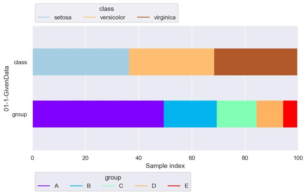

クラスラベルについては大体3等分，グループについては A から E にかけて減少していくように設定しています．

データ分割の実装例と説明

先程の一覧を上から順番に消化していきます．

check_cv

sklearn.model_selection.check_cv(cv=5, y=None, *, classifier=False)
・・・・cross-validator オブジェクト（KFold など）について確認ができます．
  - cv: cross-validator オブジェクト．int の場合は sklearn.model_selection.KFold において，何分割するかという引数の n_splits が指定できる．None の場合は KFold(n_splits=5)．
  - y: 教師あり学習における目的変数．
  - classifier: ==True でクラス分類タスクの場合は，sklearn.model_selection.StratifiedKFold が用いられます．

実装例は以下です．

from sklearn.model_selection import check_cv
print(check_cv())
# KFold(n_splits=5, random_state=None, shuffle=False)

print(check_cv(y=y, classifier=False))
# KFold(n_splits=5, random_state=None, shuffle=False)

print(check_cv(y=y, classifier=True))
# StratifiedKFold(n_splits=5, random_state=None, shuffle=False)

使った試しはありませんが，一応参考まで．

train_test_split

sklearn.model_selection.train_test_split(*arrays, test_size=None, train_size=None, random_state=None, shuffle=True, stratify=None)
・・・・学習用データと検証用データを2つに分けます（ホールド・アウト検証）．
  - *arrays: 学習用データと検証用データに分けたい元のデータで，list / numpy.ndarray, pandas.DataFrame などが指定可能．
  - test_size: 検証用データサイズを指定する．float で与える場合は 0 ～ 1 とし，元データサイズの割合として指定する．int で与える場合はデータ数を直接指定する．test_size=None, train_size=None の場合は test_size=0.25 となります．
  - train_size: 学習用データサイズを指定．他は test_size と一緒．
  - random_state: 乱数シード値を指定．
  - shuffle: データセットを分割するときに，データの順序をシャッフルするかどうかを指定．
  - stratify: データをどのラベルを用いて層化させる（学習／検証データにおいて，指定したデータラベルの割合が各データ数に対して等しくなる）かを指定．

実装例は以下です．

from sklearn.model_selection import train_test_split
train_df, test_df = train_test_split(df, test_size=0.25, shuffle=False)
print(f"train_df: shape={train_df.shape}")
print(f"train_df.index={train_df.index}")
print(f'  value counts\n{train_df["species"].value_counts()}')
print()
print(f"test_df: shape={test_df.shape}")
print(f"test_df.index={test_df.index}")
print(f'  value counts\n{test_df["species"].value_counts()}')

plotter = FoldsPlotter(x=x, y=y, group=group, ylabel="02-1-train_test_split")
plotter.add_plot(train_idx=train_df.index, test_idx=test_df.index)
plotter.show(custom_y_label=["train / test", "class", "group"])

# train_df: shape=(75, 6)
# train_df.index=Int64Index([ 0,  1,  2,  3,  4,  5,  6,  7,  8,  9, 10, 11, 12, 13, 14, 15, 16,
#             17, 18, 19, 20, 21, 22, 23, 24, 25, 26, 27, 28, 29, 30, 31, 32, 33,
#             34, 35, 36, 37, 38, 39, 40, 41, 42, 43, 44, 45, 46, 47, 48, 49, 50,
#             51, 52, 53, 54, 55, 56, 57, 58, 59, 60, 61, 62, 63, 64, 65, 66, 67,
#             68, 69, 70, 71, 72, 73, 74],
#            dtype='int64')
#   value counts
# setosa        37
# versicolor    32
# virginica      6
# Name: species, dtype: int64
# 
# test_df: shape=(25, 6)
# test_df.index=Int64Index([75, 76, 77, 78, 79, 80, 81, 82, 83, 84, 85, 86, 87, 88, 89, 90, 91,
#             92, 93, 94, 95, 96, 97, 98, 99],
#            dtype='int64')
#   value counts
# virginica    25
# Name: species, dtype: int64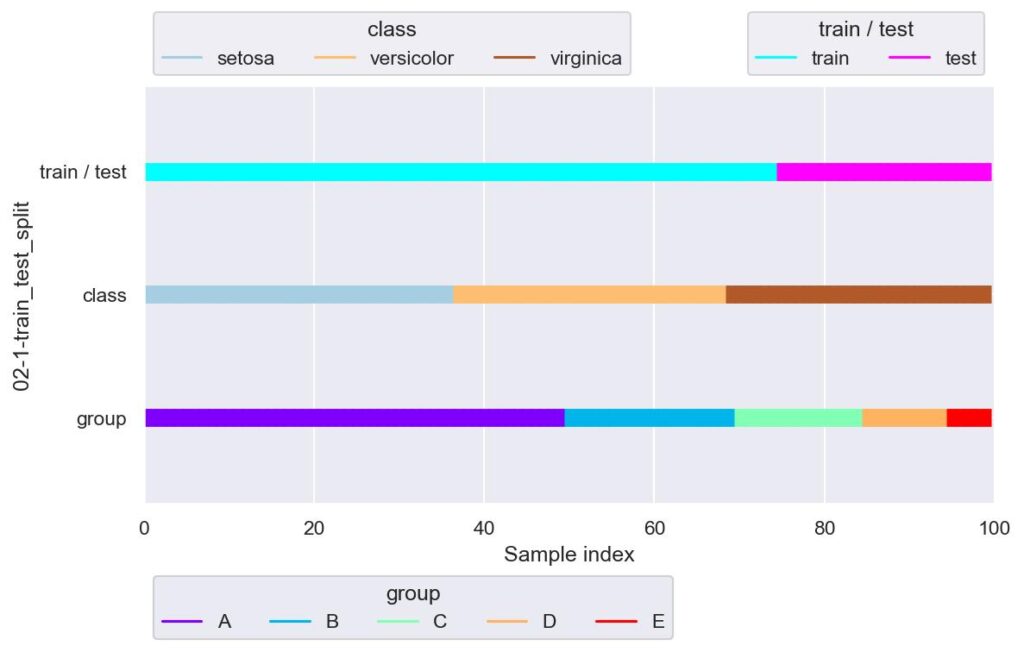

上記は検証用データのサイズを全体の 25 % とし，割り振りをランダムでなく初めから順番に取ってきた場合の出力と可視化です．
今回用意したデータはラベルとグループを名前順で整列させているので，train で表した学習用データに着目すると，virginica は 6 つのみですし，グループに至っては D, E が取得できていないなど，データ分割に偏りが生じており，不均衡なデータ分割と言えます．

split の引数で shuffle=True とすることにより，容易にある程度均衡なデータを得ることができます．

train_df, test_df = train_test_split(df, test_size=0.25, shuffle=True, random_state=0)
print("train")
print(f'  value counts\n{train_df["species"].value_counts()}')
print()
print("test")
print(f'  value counts\n{test_df["species"].value_counts()}')
plotter = FoldsPlotter(x=x, y=y, group=group, ylabel="02-2-train_test_split")
plotter.add_plot(train_idx=train_df.index, test_idx=test_df.index)
plotter.show(custom_y_label=["train / test", "class", "group"])

# train
#   value counts
# versicolor    26
# setosa        26
# virginica     23
# Name: species, dtype: int64
# 
# test
#   value counts
# setosa        11
# virginica      8
# versicolor     6
# Name: species, dtype: int64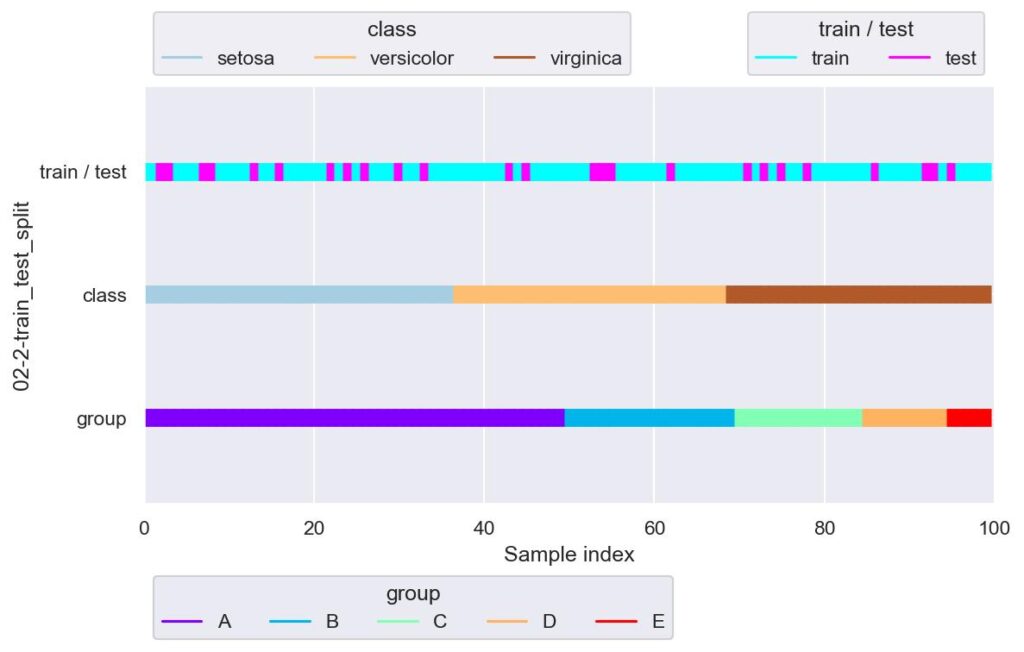

このように，学習データのラベルについては versicolor: 26, setosa: 26, virginica: 23 という具合に，まんべんなく分割できています．
可視化図では，飛び飛びの index でデータを分けていることが示されています．
注意として，データ分割の再現性を持たせたい場合は，split の引数 random_state を設定するのをお忘れなく．

また，割合を適用するデータについて split の引数 stratify で指定することができ，ここにラベルを指定することで，train_size / test_size に指定した割合で各ラベルのデータを分割することができます．

train_df, test_df = train_test_split(df, test_size=0.25, shuffle=True, random_state=0, stratify=y)
print("train")
print(f'  value counts\n{train_df["species"].value_counts()}')
print()
print("test")
print(f'  value counts\n{test_df["species"].value_counts()}')
plotter = FoldsPlotter(x=x, y=y, group=group, ylabel="02-3-train_test_split")
plotter.add_plot(train_idx=train_df.index, test_idx=test_df.index)
plotter.show(custom_y_label=["train / test", "class", "group"])

# train
#   value counts
# setosa        28
# versicolor    24
# virginica     23
# Name: species, dtype: int64
# 
# test
#   value counts
# setosa        9
# virginica     8
# versicolor    8
# Name: species, dtype: int64

test_size=0.25 としているので，train : test = 3 : 1 にデータ分割されますが，例えば setosa だと train : test = 28 : 9 というふうに各ラベルについても 3 : 1 でデータ分割することができます．

train_test_split の初めに与える引数について，上の例ではデータセット全体を渡していましたが，説明変数と目的変数を分けて与えることで，説明変数と目的変数の別々の戻り値を取得することができます（個人的には，たまに戻り値の順番が train-train-test-test だと勘違いします）．

train_x, test_x, train_y, test_y = train_test_split(
    x, y,
    test_size=0.25, shuffle=True, random_state=0, stratify=y
)
print(f"train_x.shape={train_x.shape}, train_y.shape={train_y.shape}")
print()
print(f"test_x.shape={test_x.shape}, test_y.shape={test_y.shape}")
plotter = FoldsPlotter(x=x, y=y, group=group, ylabel="02-4-train_test_split")
plotter.add_plot(train_idx=train_x.index, test_idx=test_x.index)
plotter.show(custom_y_label=["train / test", "class", "group"])

# train_x.shape=(75, 5), train_y.shape=(75,)
# test_x.shape=(25, 5), test_y.shape=(25,)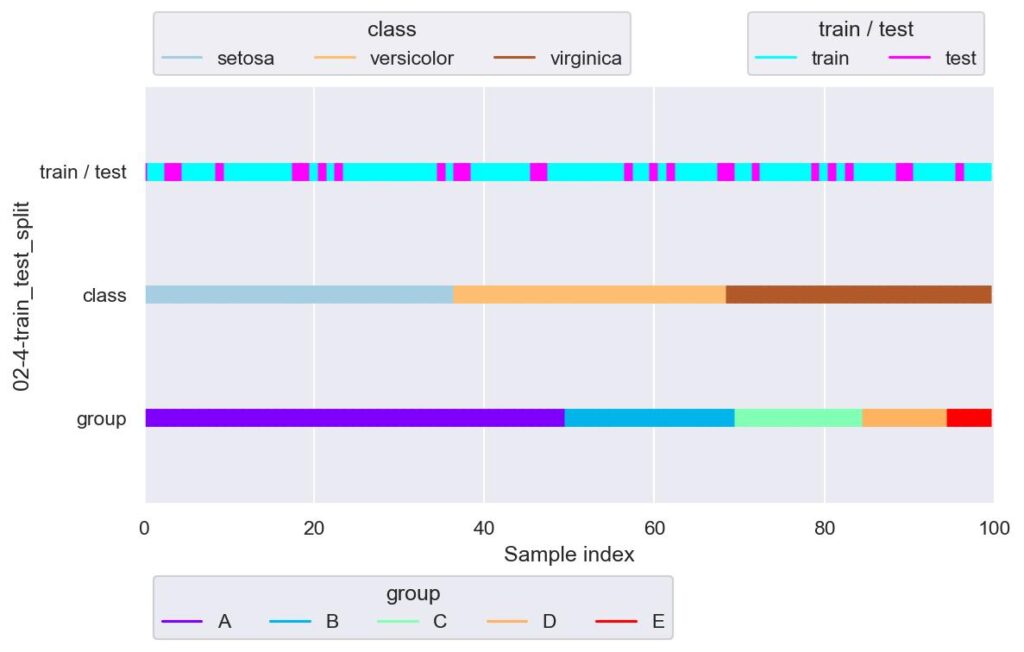

stratify で指定するデータの種類よりも test_size が小さいとエラーが送出されます．

# train_x, test_x, train_y, test_y = train_test_split(
#     x, y,
#     test_size=2, shuffle=True, random_state=0, stratify=y
# )

# ValueError: The test_size = 2 should be greater or equal to the number of classes = 3

KFold

sklearn.model_selection.KFold(n_splits=5, *, shuffle=False, random_state=None)
・・・・データを指定した K 個に等分し，1 つを検証用，それ以外の K-1 個を学習に用います．各 fold における検証用データには重複させないようにします．
  - n_splits: データを何等分するかを指定できます．
  - shuffle: True の場合にデータを抽出する際に元データの順番を保持せず，ランダムなインデックスで抽出します．
  - random_state: 上記ランダム抽出に用いる乱数シードを設定します．

実装例は以下です．

from sklearn.model_selection import KFold

kf = KFold(n_splits=5, shuffle=True, random_state=42)
plotter = FoldsPlotter(x=x, y=y, group=group, ylabel="03-1-KFold")
for i, (train_idx, test_idx) in enumerate(kf.split(X=x, y=y, groups=group)):
    print(f"\nfold-{i}")
    print(f"train_idx.shape={train_idx.shape}, test_idx.shape={test_idx.shape}")
    print(f"set(y.iloc[test_idx])={set(y.iloc[test_idx])}")
    print(f"train_idx={train_idx}")
    print(f"test_idx={test_idx}")
    plotter.add_plot(train_idx=train_idx, test_idx=test_idx)
plotter.show()

# fold-0
# train_idx.shape=(80,), test_idx.shape=(20,)
# set(y.iloc[test_idx])={'virginica', 'setosa', 'versicolor'}
# train_idx=[ 1  2  3  5  6  7  8  9 11 13 14 15 16 17 19 20 21 23 24 25 26 27 28 29
#  32 34 35 36 37 38 40 41 42 43 46 47 48 49 50 51 52 54 55 56 57 58 59 60
#  61 62 63 64 65 66 67 68 69 71 72 74 75 78 79 81 82 84 85 86 87 88 89 91
#  92 93 94 95 96 97 98 99]
# test_idx=[ 0  4 10 12 18 22 30 31 33 39 44 45 53 70 73 76 77 80 83 90]
# 
# fold-1
# train_idx.shape=(80,), test_idx.shape=(20,)
# set(y.iloc[test_idx])={'virginica', 'setosa', 'versicolor'}
# train_idx=[ 0  1  2  3  4  6  7  8 10 12 13 14 17 18 19 20 21 22 23 24 25 27 29 30
#  31 32 33 34 36 37 38 39 41 43 44 45 46 48 49 50 51 52 53 54 56 57 58 59
#  60 61 62 63 64 67 68 70 71 73 74 75 76 77 78 79 80 81 82 83 84 86 87 89
#  90 91 92 94 95 97 98 99]
# test_idx=[ 5  9 11 15 16 26 28 35 40 42 47 55 65 66 69 72 85 88 93 96]
# 
# fold-2
# train_idx.shape=(80,), test_idx.shape=(20,)
# set(y.iloc[test_idx])={'virginica', 'setosa', 'versicolor'}
# train_idx=[ 0  1  2  4  5  9 10 11 12 14 15 16 18 20 21 22 23 26 28 29 30 31 32 33
#  35 37 39 40 41 42 43 44 45 46 47 48 50 51 52 53 54 55 56 57 58 59 60 61
#  63 65 66 67 68 69 70 71 72 73 74 75 76 77 79 80 82 83 84 85 86 87 88 90
#  91 92 93 94 96 97 98 99]
# test_idx=[ 3  6  7  8 13 17 19 24 25 27 34 36 38 49 62 64 78 81 89 95]
# 
# fold-3
# train_idx.shape=(80,), test_idx.shape=(20,)
# set(y.iloc[test_idx])={'virginica', 'setosa', 'versicolor'}
# train_idx=[ 0  1  2  3  4  5  6  7  8  9 10 11 12 13 14 15 16 17 18 19 20 21 22 23
#  24 25 26 27 28 29 30 31 33 34 35 36 37 38 39 40 42 44 45 47 49 51 52 53
#  55 60 62 63 64 65 66 69 70 71 72 73 74 76 77 78 80 81 82 83 84 85 86 87
#  88 89 90 91 92 93 95 96]
# test_idx=[32 41 43 46 48 50 54 56 57 58 59 61 67 68 75 79 94 97 98 99]
# 
# fold-4
# train_idx.shape=(80,), test_idx.shape=(20,)
# set(y.iloc[test_idx])={'virginica', 'setosa', 'versicolor'}
# train_idx=[ 0  3  4  5  6  7  8  9 10 11 12 13 15 16 17 18 19 22 24 25 26 27 28 30
#  31 32 33 34 35 36 38 39 40 41 42 43 44 45 46 47 48 49 50 53 54 55 56 57
#  58 59 61 62 64 65 66 67 68 69 70 72 73 75 76 77 78 79 80 81 83 85 88 89
#  90 93 94 95 96 97 98 99]
# test_idx=[ 1  2 14 20 21 23 29 37 51 52 60 63 71 74 82 84 86 87 91 92]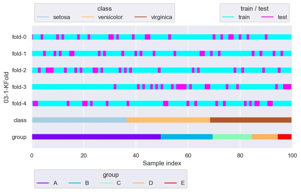

fold-3 において，setosa の検証用データが少ないように見えます．
shuffle = True としているので見ずらいですが，各 fold において検証用データの index は重複していません．
見やすくするために shuffle = False としたのが次です．

kf = KFold(n_splits=5, shuffle=False)
plotter = FoldsPlotter(x=x, y=y, group=group, ylabel="03-2-KFold")
for i, (train_idx, test_idx) in enumerate(kf.split(X=x)):
    plotter.add_plot(train_idx=train_idx, test_idx=test_idx)
plotter.show()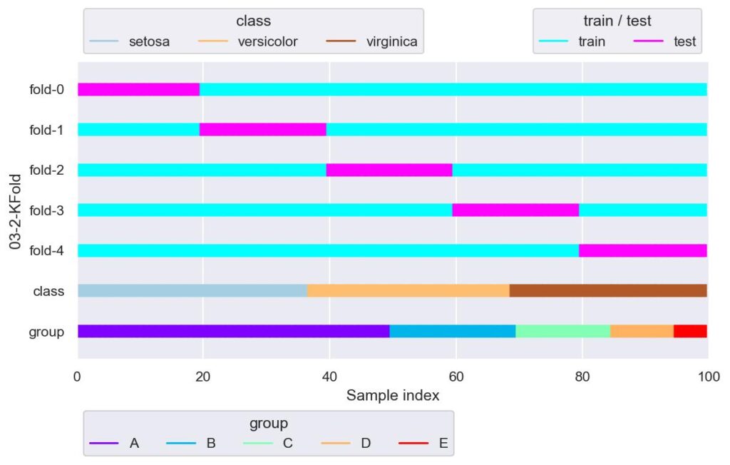

この通り，各 fold における検証用データの index の重複はないことが示されています．
しかし，index に対してラベルが順番で整列されている今回のデータにおいては，KFold を用いる場合は shuffle = True としないと，上図のようにデータが偏ります．
ラベルの個数が偏らないようにするためには，StratifiedKFold（後述）を用います．

ShuffleSplit

sklearn.model_selection.ShuffleSplit(n_splits=10, *, test_size=None, train_size=None, random_state=None)
・・・・train_test.split(shuffle=True, stratify=None) を複数回作用させるような学習用／検証用データのインデックスを返すオブジェクトを生成します．各 fold における検証用データは重複します．
  - n_splits: 学習用／検証用データセットのインデックスを何回返すかを指定します．
  - test_size: 検証用データセットの割合を指定します．
  - train_size: 学習用データセットの割合を指定します．
  - random_state: ランダム抽出に用いる乱数シードを設定します．

実装例は以下です．

from sklearn.model_selection import ShuffleSplit

ss = ShuffleSplit(n_splits=2, test_size=0.5, random_state=42)
plotter = FoldsPlotter(x=x, y=y, group=group, ylabel="04-1-ShuffleSplit")
for i, (train_idx, test_idx) in enumerate(ss.split(X=x)):
    plotter.add_plot(train_idx=train_idx, test_idx=test_idx)
plotter.show()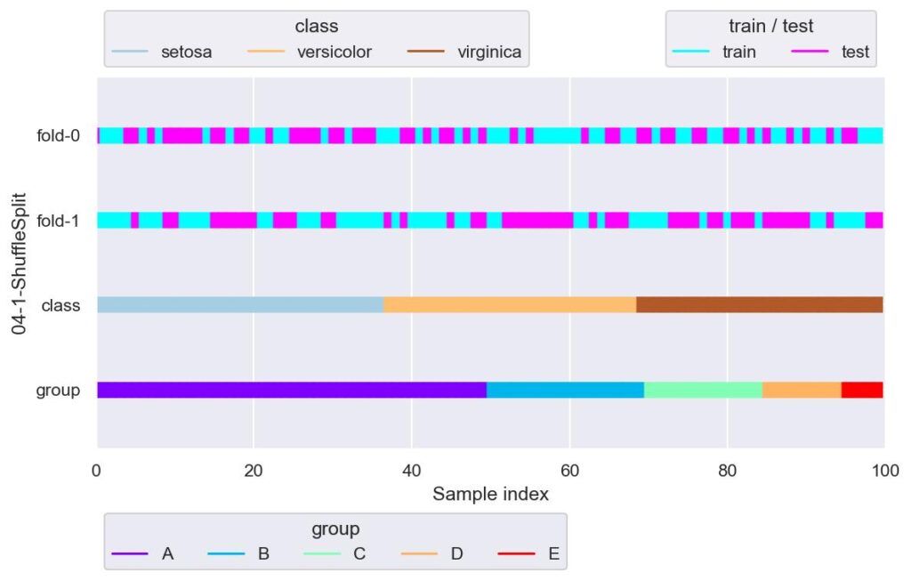

各 fold でそれぞれ独立して train_test_split(stratify=None, shuffle=True) を行っています．

StratifiedKFold

sklearn.model_selection.StratifiedKFold(n_splits=5, *, shuffle=False, random_state=None)
・・・・データを指定した K 個に等分し，1 つを検証用，それ以外の K-1 個を学習に用います．データ分割の際には，メソッド split の引数 y にてラベルやグループを指定することにより，全種類のラベルも均等に分割されます．各 fold における検証用データに重複はさせないようにします．
  - n_splits: データを何等分するかを指定できます．
  - shuffle: True の場合にデータを抽出する際に元データの順番を保持せず，ランダムなインデックスで抽出します．
  - random_state: 上記ランダム抽出に用いる乱数シードを設定します．

実装例は以下です．

from sklearn.model_selection import StratifiedKFold

skf = StratifiedKFold(n_splits=3, shuffle=False)
plotter = FoldsPlotter(x=x, y=y, group=group, ylabel="05-1-StratifiedKFold")
for i, (train_idx, test_idx) in enumerate(skf.split(X=x, y=y)):
    print(f"\nfold-{i}")
    print(f'  y[test_idx].value_counts()\n{y[test_idx].value_counts()}')
    plotter.add_plot(train_idx=train_idx, test_idx=test_idx)
plotter.show()

# fold-0
#   y[test_idx].value_counts()
# setosa        13
# virginica     11
# versicolor    10
# Name: species, dtype: int64
# 
# fold-1
#   y[test_idx].value_counts()
# setosa        12
# versicolor    11
# virginica     10
# Name: species, dtype: int64
# 
# fold-2
#   y[test_idx].value_counts()
# setosa        12
# versicolor    11
# virginica     10
# Name: species, dtype: int64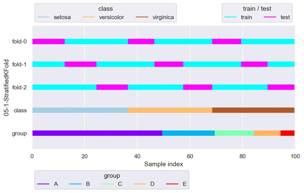

ラベルの個数を各 fold で均等に分けながら，KFold を行います．
学習のときに用いることができるデータセットと本番実装後における実際のデータの相関がほとんど同じであれば，有力なデータ分割手法と言えるでしょう．

skf = StratifiedKFold(n_splits=3, shuffle=True, random_state=True)
plotter = FoldsPlotter(x=x, y=y, group=group, ylabel="05-2-StratifiedKFold")
for i, (train_idx, test_idx) in enumerate(skf.split(X=x, y=y)):
    plotter.add_plot(train_idx=train_idx, test_idx=test_idx)
plotter.show()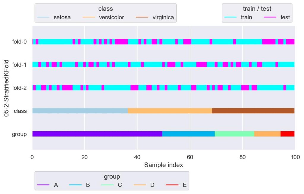

元データにおいて，index が意図せずデータに関係してしまうのであれば，shuffle = True としたほうが良いでしょう．

StratifiedShuffleSplit

sklearn.model_selection.StratifiedShuffleSplit(n_splits=10, *, test_size=None, train_size=None, random_state=None)
・・・・train_test.split(shuffle=True, stratify=y) を複数回作用させるような学習用／検証用データのインデックスを返すオブジェクトを生成します．各 fold における検証用データは重複します．
  - n_splits: 学習用／検証用データセットのインデックスを何回返すかを指定します．
  - test_size: 検証用データセットの割合を指定します．
  - train_size: 学習用データセットの割合を指定します．
  - random_state: ランダム抽出に用いる乱数シードを設定します．

実装例は以下です．

from sklearn.model_selection import StratifiedShuffleSplit

sss = StratifiedShuffleSplit(n_splits=2, test_size=0.25, random_state=42)
plotter = FoldsPlotter(x=x, y=y, group=group, ylabel="06-1-StratifiedShuffleSplit")
for i, (train_idx, test_idx) in enumerate(sss.split(X=x, y=y)):
    print(f"\nfold-{i}")
    print(f'  y[test_idx].value_counts()\n{y[test_idx].value_counts()}')
    plotter.add_plot(train_idx, test_idx)
plotter.show()

# fold-0
#   y[test_idx].value_counts()
# setosa        9
# versicolor    8
# virginica     8
# Name: species, dtype: int64
# 
# fold-1
#   y[test_idx].value_counts()
# setosa        9
# versicolor    8
# virginica     8
# Name: species, dtype: int64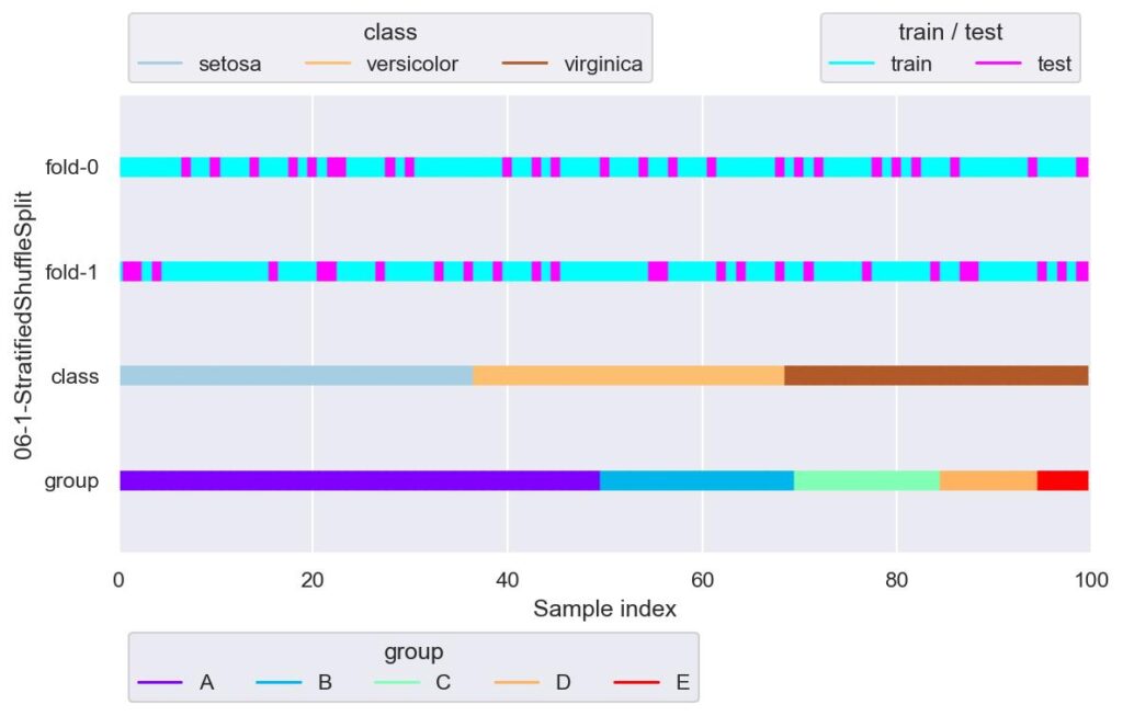

各 fold にて独立して，train_test_split(stratify={label data}, shuffle=True) を n_splits 回行います．

sss = StratifiedShuffleSplit(n_splits=5, test_size=0.25, random_state=42)
plotter = FoldsPlotter(x=x, y=y, group=group, ylabel="06-2-StratifiedShuffleSplit")
for i, (train_idx, test_idx) in enumerate(sss.split(X=x, y=y)):
    plotter.add_plot(train_idx, test_idx)
plotter.show()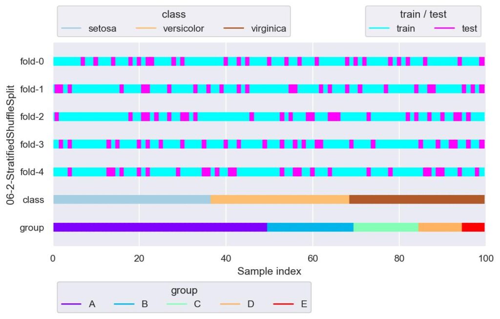

GroupKFold

sklearn.model_selection.GroupKFold(n_splits=5)
・・・・データを指定した K 個に分割し，1 つを検証用，それ以外の K-1 個を学習に用います．データ分割の際には，メソッド split の引数 groups にて指定したグループによって，分割するインデックスを制御します．各 fold における検証用データに重複させないようにします．
  - n_splits: データを何分割するかを指定できます．

実装例は以下です．

from sklearn.model_selection import GroupKFold

# gkf = GroupKFold(n_splits=10)
# for train_idx, test_idx in gkf.split(X=x, y=y, groups=group):
#     print(train_idx.shape, test_idx.shape)
#
# ValueError: Cannot have number of splits n_splits=10 greater than the number of groups: 5.

今回，group には架空のデータである area を設定していて，set(area) = {"A", "B", "C", "D", "E"} の 5 種類としています．
上記のエラーは，この 5 種類よりも多く分割しようとしているため，エラーが送出されています．

gkf = GroupKFold(n_splits=3)
plotter = FoldsPlotter(x=x, y=y, group=group, ylabel="07-1-GroupKFold")
for i, (train_idx, test_idx) in enumerate(gkf.split(X=x, y=y, groups=group)):
    plotter.add_plot(train_idx, test_idx)
plotter.show()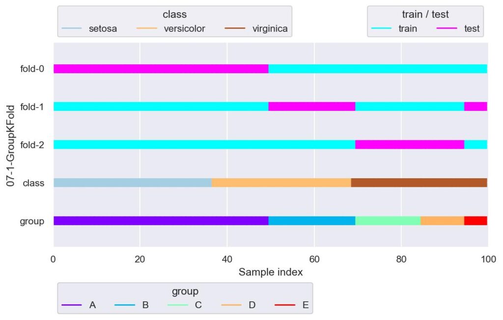

一番下がグループの分割を表していますが，これに沿って n_splits で指定した個数の 3 つに学習用データと検証用データが分けられています．
しかし上記の例だと，目的変数であるラベルについて，fold-0 は virginica について学習できていません．

gkf = GroupKFold(n_splits=len(set(group)))
plotter = FoldsPlotter(x=x, y=y, group=group, ylabel="07-2-GroupKFold")
for i, (train_idx, test_idx) in enumerate(gkf.split(X=x, y=y, groups=group)):
    plotter.add_plot(train_idx, test_idx)
plotter.show()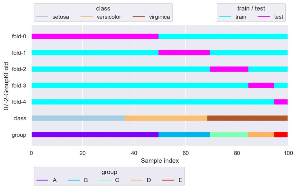

上図はグループごとにデータ分割した例です．
先ほどと同様，fold-0 では verginica が学習できてないですね．

GroupShuffleSplit

sklearn.model_selection.GroupShuffleSplit(n_splits=5, *, test_size=None, train_size=None, random_state=None)
・・・・GroupKFold のデータ分割で，各 fold 間におけるグループの重複を許したデータ分割手法．
  - n_splits: 学習用／検証用データセットのインデックスを何回返すかを指定します．
  - test_size: 検証用データセットの割合を指定します．
  - train_size: 学習用データセットの割合を指定します．
  - random_state: ランダム抽出に用いる乱数シードを設定します．

実装例は以下です．

from sklearn.model_selection import GroupShuffleSplit

gss = GroupShuffleSplit(n_splits=10, random_state=42)
plotter = FoldsPlotter(x=x, y=y, group=group, ylabel="08-1-GroupShuffleSplit")
for i, (train_idx, test_idx) in enumerate(gss.split(X=x, y=y, groups=group)):
    plotter.add_plot(train_idx, test_idx)
plotter.show()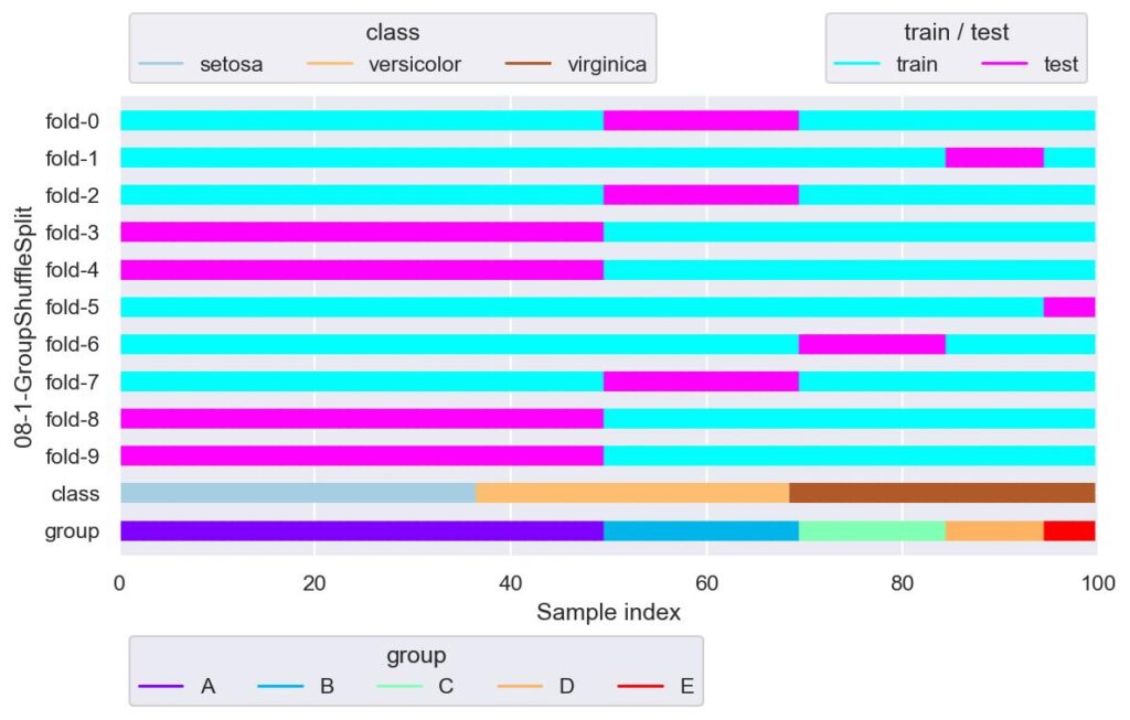

グループが少ないと，同じ分割の fold が多数存在しています．

gss = GroupShuffleSplit(n_splits=2, test_size=0.25, random_state=42)
plotter = FoldsPlotter(x=x, y=y, group=group, ylabel="08-2-GroupShuffleSplit")
for i, (train_idx, test_idx) in enumerate(gss.split(X=x, y=y, groups=x["area"])):
    plotter.add_plot(train_idx, test_idx)
plotter.show()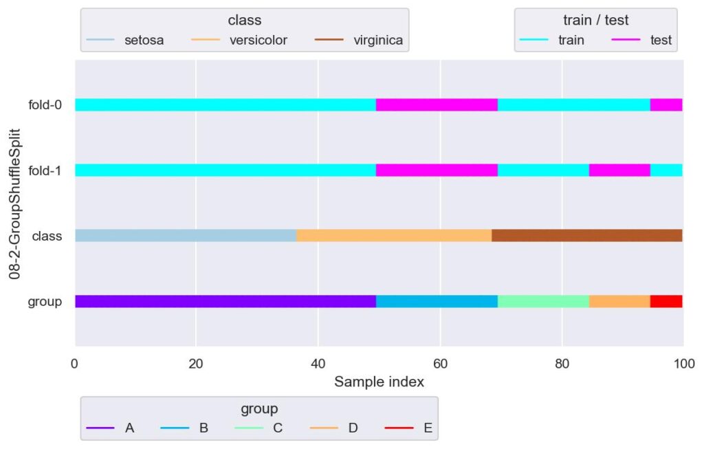

目的変数がラベルであるクラス分類の場合，層化分割しない（stratified じゃない）ようなグループによる分割は，全部の種類のラベルが学習できなかったり，あるいは重複したりする fold が現れるため，適していないように思えます．

StratifiedGroupKFold

sklearn.model_selection.StratifiedGroupKFold(n_splits=5, shuffle=False, random_state=None)
・・・・データを指定した K 個に分割し，1 つを検証用，それ以外の K-1 個を学習に用います．データ分割は，メソッド split の引数 y にて指定したラベル，groups にて指定したグループを用いて，グループのまとまりを使ってラベルを K 個に均等に分けるように作用します．イメージとしては，名前の通り StratifiedKFold と GroupKFold が合体したものです．各 fold における検証用データのグループは重複しません．
  - n_splits: データを何分割するかを指定できます．
  - shuffle: True の場合にデータを抽出する際に元データの順番を保持せず，ランダムなインデックスで抽出します．
  - random_state: 上記ランダム抽出に用いる乱数シードを設定します．

実装例は以下です．

from sklearn.model_selection import StratifiedGroupKFold

sgkf = StratifiedGroupKFold(n_splits=3, shuffle=True, random_state=42)
plotter = FoldsPlotter(x=x, y=y, group=group, ylabel="09-1-StratifiedGroupKFold")
for i, (train_idx, test_idx) in enumerate(sgkf.split(X=x, y=y, groups=group)):
    plotter.add_plot(train_idx, test_idx)
plotter.show()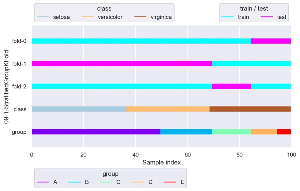

グループによってラベルを均等に分割しようと試みていますが，今回のデータはラベルもグループも種類が少ないので，ほぼ GroupKFold のような結果になっています．

sgkf = StratifiedGroupKFold(n_splits=10, shuffle=False)
plotter = FoldsPlotter(x=x, y=y, group=group, ylabel="09-2-StratifiedGroupKFold")
for i, (train_idx, test_idx) in enumerate(sgkf.split(X=x, y=y, groups=group)):
    plotter.add_plot(train_idx, test_idx)
plotter.show()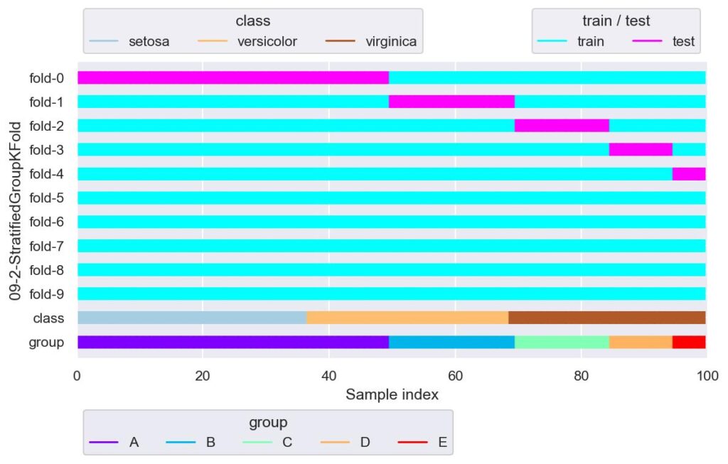

仮にグループ数よりも n_splits を大きくすると，グループ数を越えた fold から，検証用データが全く割り当てられないという結果になりました．

sgkf = StratifiedGroupKFold(n_splits=2, shuffle=True)
plotter = FoldsPlotter(x=x, y=y, group=group, ylabel="09-3-StratifiedGroupKFold")
for i, (train_idx, test_idx) in enumerate(sgkf.split(X=x, y=y, groups=group)):
    plotter.add_plot(train_idx, test_idx)
plotter.show()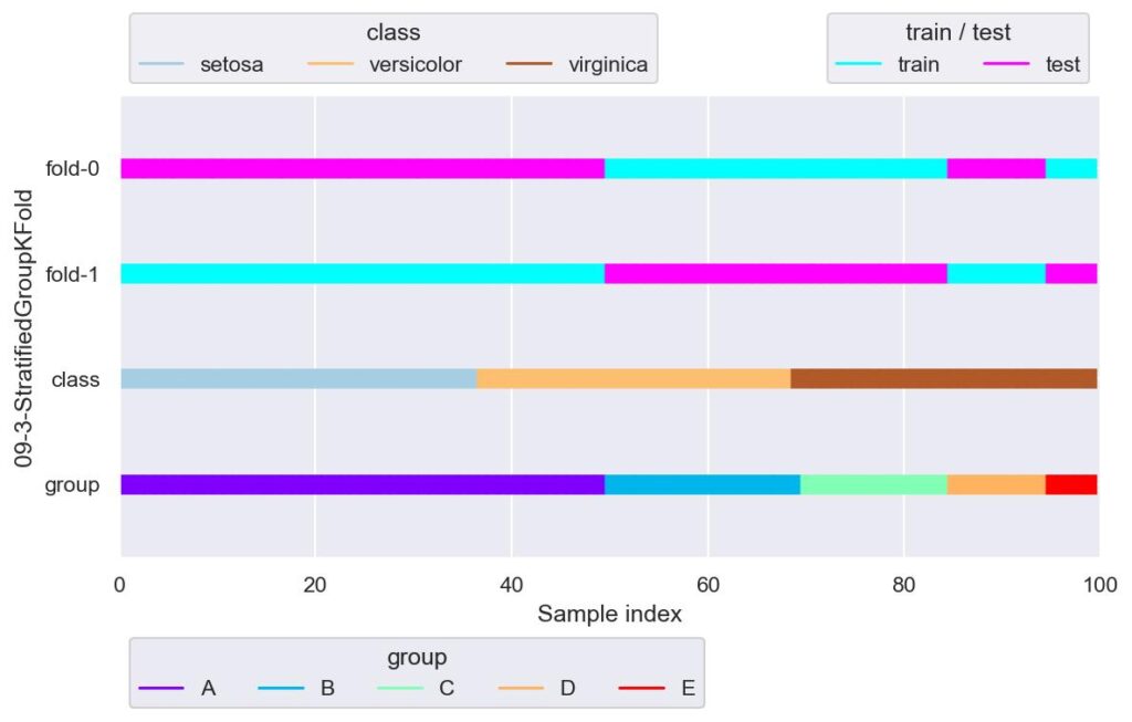

今回のデータでは，StratifiedGroupKFold を用いてまともにデータ分割しようとすると，n_splits=2 くらいしか使えそうにありません．
このように，学習用／検証用データ，あるいは本番実装を模して残しておいたデータについて，データが不均衡でないか可視化を行うことは重要と言えます．

RepeatedKFold

sklearn.model_selection.RepeatedKFold(*, n_splits=5, n_repeats=10, random_state=None)
・・・・KFold を n_repeats で指定した回数分行います．リピートされる各 fold 間では検証用データの重複はありませんが，各リピート間では検証用データの重複は発生します．
  - n_splits: データを何分割するかを指定できます．
  - n_repeats: KFold を繰り返す回数を指定します．
  - random_state: ランダム抽出に用いる乱数シードを設定します．

実装例は以下です．

from sklearn.model_selection import RepeatedKFold

rkf = RepeatedKFold(n_splits=3, n_repeats=3, random_state=42)
plotter = FoldsPlotter(x=x, y=y, group=group, ylabel="10-1-RepeatedKFold")
for i, (train_idx, test_idx) in enumerate(rkf.split(X=x, y=y, groups=group)):
    plotter.add_plot(train_idx, test_idx)
plotter.show()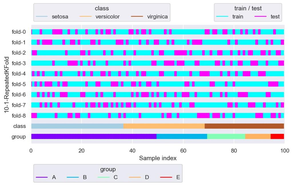

n_splits=3 としており，fold-0 ～ fold-2, fold-3 ～ fold-5, fold-6 ～ fold-8 において検証用データの重複はありません．

RepeatedStratifiedKFold

sklearn.model_selection.RepeatedStratifiedKFold(*, n_splits=5, n_repeats=10, random_state=None)
・・・・StratifiedKFold を n_repeats で指定した回数分行います．リピートされる各 fold 間では検証用データの重複はありませんが，各リピート間では検証用データの重複は発生します．
  - n_splits: データを何分割するかを指定できます．
  - n_repeats: KFold を繰り返す回数を指定します．
  - random_state: ランダム抽出に用いる乱数シードを設定します．

実装例は以下です．

from sklearn.model_selection import RepeatedStratifiedKFold

rskf = RepeatedStratifiedKFold(n_splits=2, n_repeats=2, random_state=42)
plotter = FoldsPlotter(x=x, y=y, group=group, ylabel="11-1-RepeatedStratifiedKFold")
for i, (train_idx, test_idx) in enumerate(rskf.split(X=x, y=y, groups=group)):
    plotter.add_plot(train_idx, test_idx)
plotter.show()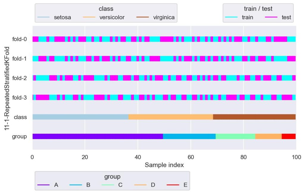

StratifiedKFold にて，データの重複があっても良いから更に色んな分割で試してみたいときとかに使う感じでしょうか．

rskf = RepeatedStratifiedKFold(n_splits=3, n_repeats=3, random_state=42)
plotter = FoldsPlotter(x=x, y=y, group=group, ylabel="11-2-RepeatedStratifiedKFold")
for i, (train_idx, test_idx) in enumerate(rskf.split(X=x, y=y, groups=group)):
    plotter.add_plot(train_idx, test_idx)
plotter.show()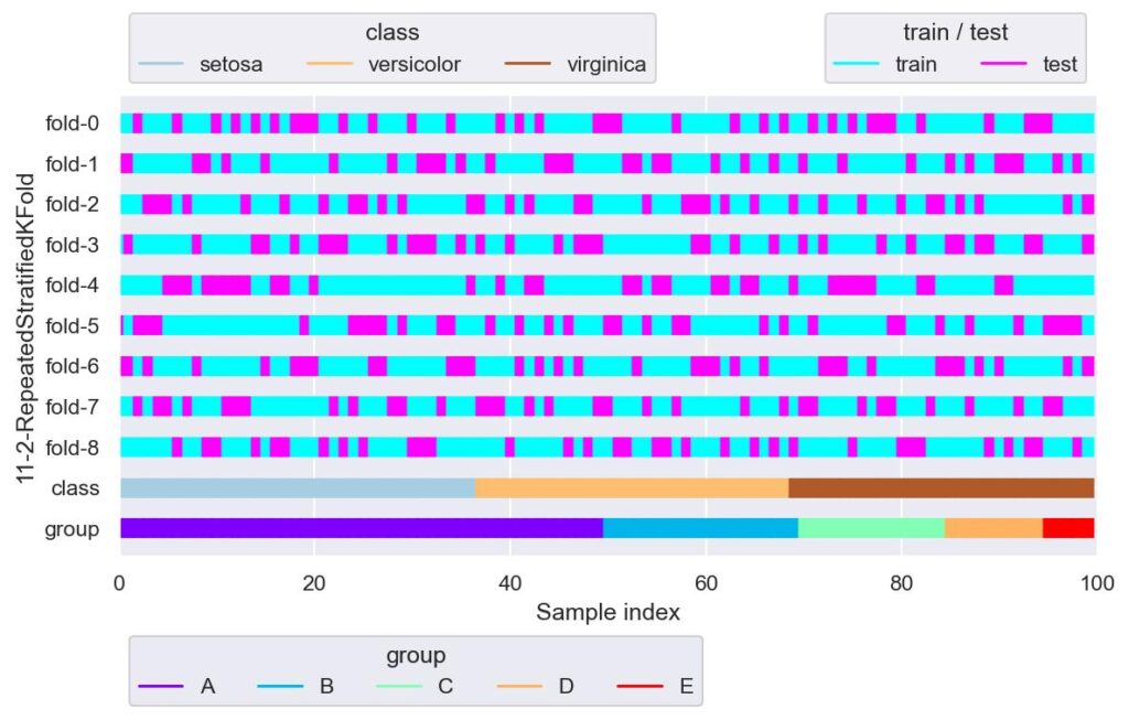

LeaveOneOut

sklearn.model_selection.LeaveOneOut()
・・・・一つだけを検証用データ，その他は学習用データとして分割します．

実装例は以下です．

from sklearn.model_selection import LeaveOneOut

loo = LeaveOneOut()
plotter = FoldsPlotter(x=x, y=y, group=group, ylabel="12-1-LeaveOneOut")
for i, (train_idx, test_idx) in enumerate(loo.split(X=x, y=y, groups=group)):
    plotter.add_plot(train_idx, test_idx)
plotter.show()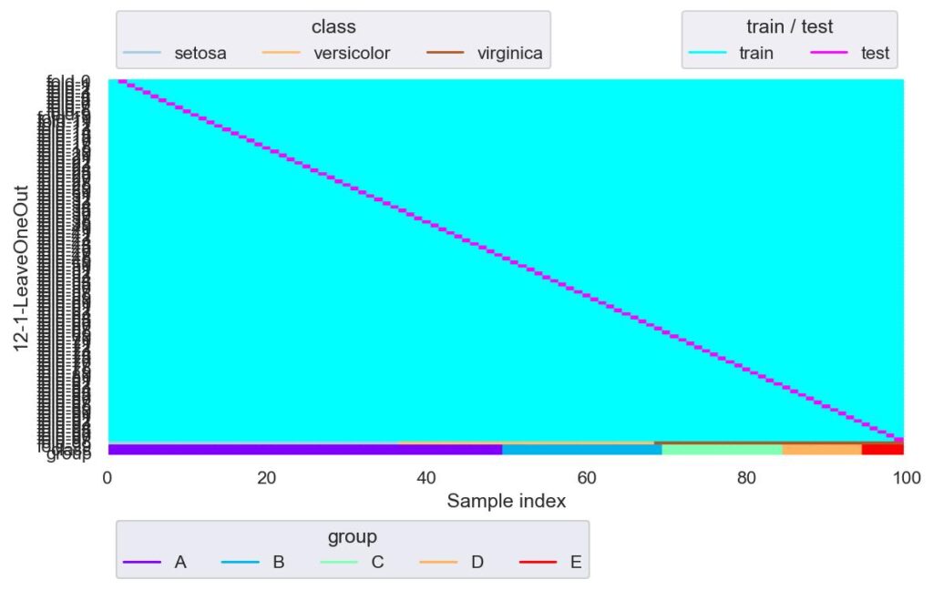

一つのみを検証用データとしそれ以外は学習用データとするので，fold はデータ数分できます．
データが極端に少ないときに有効かと思われますが，その場合は，きちんとデータを集めたほうが汎化性能は高いでしょう．

print(f"train_idx={train_idx}")
print(f"test_idx={test_idx}")

# train_idx=[ 0  1  2  3  4  5  6  7  8  9 10 11 12 13 14 15 16 17 18 19 20 21 22 23
#  24 25 26 27 28 29 30 31 32 33 34 35 36 37 38 39 40 41 42 43 44 45 46 47
#  48 49 50 51 52 53 54 55 56 57 58 59 60 61 62 63 64 65 66 67 68 69 70 71
#  72 73 74 75 76 77 78 79 80 81 82 83 84 85 86 87 88 89 90 91 92 93 94 95
#  96 97 98]
# test_idx=[99]

LeavePOut

sklearn.model_selection.LeavePOut(p)
・・・・引数 p で指定した個数を検証用データ，その他を学習用データとして分割します．検証用データが複数の場合は，検証用データの組み合わせが各 fold にて重複しないように，網羅的に fold が設定されます．例えば，データ数が m 個，引数 p を n 個と設定すると，総 fold 数は数学の組み合わせの記号 C を用いて，mCn = m*(m-1) / (n*(n-1)) 個生成されます．
  - p: 検証用データの個数を指定します．

実装例は以下です．

from sklearn.model_selection import LeavePOut

lpo = LeavePOut(p=1)
plotter = FoldsPlotter(x=x, y=y, group=group, ylabel="13-1-LeavePOut")
for i, (train_idx, test_idx) in enumerate(lpo.split(X=x, y=y, groups=group)):
    plotter.add_plot(train_idx, test_idx)
plotter.show()

p=1 の場合は LeaveOneOut と同じになります．

lpo = LeavePOut(p=2)
plotter = FoldsPlotter(x=x, y=y, group=group, ylabel="13-2-LeavePOut")
for i, (train_idx, test_idx) in enumerate(lpo.split(X=x, y=y, groups=group)):
    plotter.add_plot(train_idx, test_idx)
plotter.show()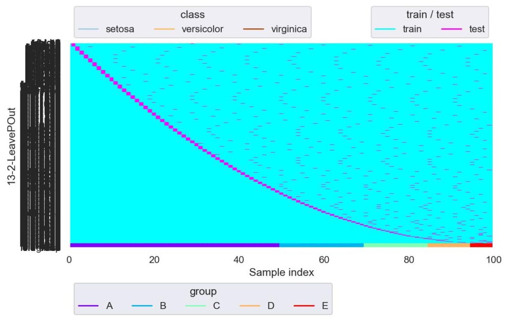

縦軸の軸ラベルが被って潰れるほど fold 数が凄まじくなっています．
LeavePOut の fold 数はデータ数が m 個，引数 p を n 個と設定すると，総 fold 数は数学の組み合わせの記号 C を用いて，mCn = m*(m-1) / (n*(n-1)) 個生成されます．
確認するために，以下で計算してみました．

lpo = LeavePOut(p=2)
for i, (train_idx, test_idx) in enumerate(lpo.split(X=x, y=y, groups=group)):
    pass
print(i)
# 4949

int(100*99 / (2*1)) - 1
# 4949

lpo = LeavePOut(p=3)
for i, (train_idx, test_idx) in enumerate(lpo.split(X=x, y=y, groups=group)):
    pass
print(i)
# 161699

int(100*99*98 / (3*2*1)) - 1
# 161699

LeaveOneGroupOut

sklearn.model_selection.LeaveOneGroupOut()
・・・・1 つのグループを検証用データとし，それ以外を学習用データとして分割します．

実装例は以下です．

from sklearn.model_selection import LeaveOneGroupOut

logo = LeaveOneGroupOut()
plotter = FoldsPlotter(x=x, y=y, group=group, ylabel="14-1-LeaveOneGroupOut")
for i, (train_idx, test_idx) in enumerate(logo.split(X=x, y=y, groups=group)):
    plotter.add_plot(train_idx, test_idx)
plotter.show()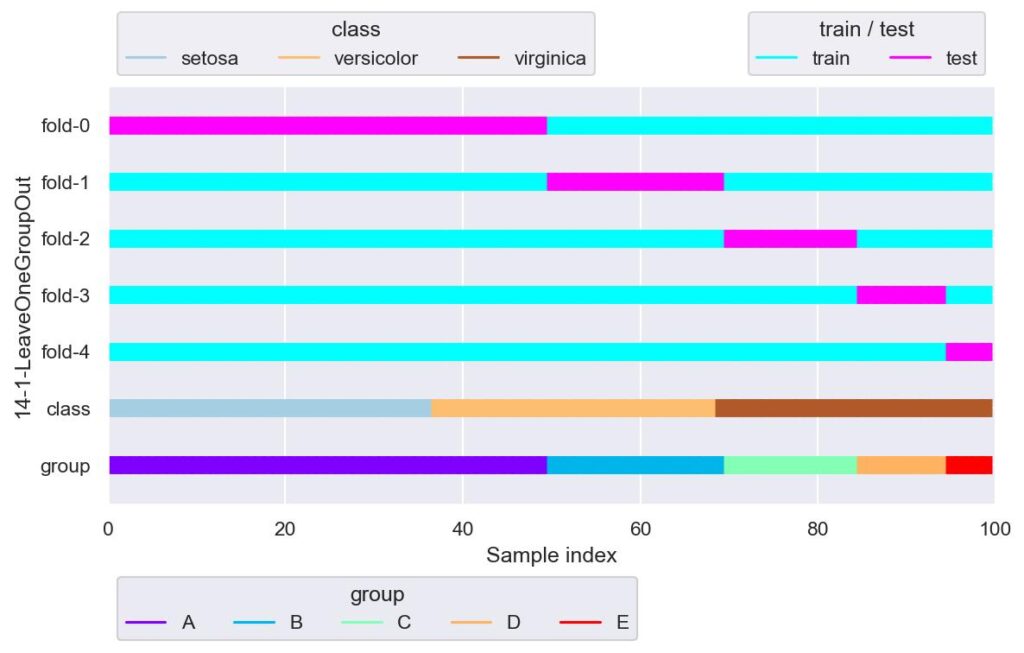

グループ一つのみを検証用データ，それ以外を学習用データとして分割します．
GroupKFold で n_splits をグループ数としたときと同等です．

LeavePGroupsOut

sklearn.model_selection.LeavePGroupsOut(n_groups)
・・・・引数 n_groups で指定したグループ数を検証用データ，その他を学習用データとして分割します．検証用データが複数の場合は，検証用データの組み合わせが各 fold にて重複しないように，網羅的に fold が設定されます．例えば，グループ数が m 個，引数 n_groups を n 個と設定すると，総 fold 数は数学の組み合わせの記号 C を用いて，mCn = m*(m-1) / (n*(n-1)) 個生成されます．
  - n_groups: 検証用データの個数を指定します．

実装例は以下です．

from sklearn.model_selection import LeavePGroupsOut

lpgo = LeavePGroupsOut(n_groups=1)
plotter = FoldsPlotter(x=x, y=y, group=group, ylabel="15-1-LeavePGroupsOut")
for i, (train_idx, test_idx) in enumerate(lpgo.split(X=x, y=y, groups=group)):
    plotter.add_plot(train_idx, test_idx)
plotter.show()

n_groups=1 の場合は LeaveOneGroupOut と同等です．

lpgo = LeavePGroupsOut(n_groups=3)
plotter = FoldsPlotter(x=x, y=y, group=group, ylabel="15-2-LeavePGroupsOut")
for i, (train_idx, test_idx) in enumerate(lpgo.split(X=x, y=y, groups=group)):
    plotter.add_plot(train_idx, test_idx)
plotter.show()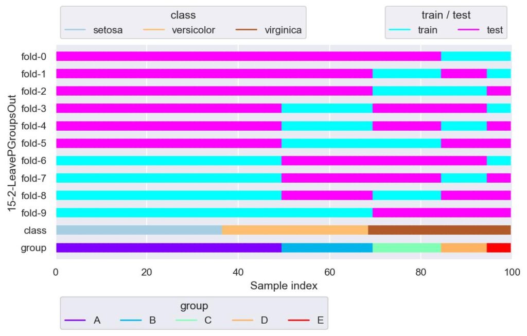

データ数がそれなりだと LeavePOut の適用はまず候補から外れますが，グループ数がそこまで多くなければ LeavePGroupsOut も良いかもしれません．

n_groups にグループ数よりも大きい値を入れると，エラーが送出されます．

# lpgo = LeavePGroupsOut(n_groups=10)
# for i, (train_idx, test_idx) in enumerate(lpgo.split(X=x, y=y, groups=group)):
    # pass

# ValueError: The groups parameter contains fewer than (or equal to) n_groups (10) numbers of unique groups (['A' 'B' 'C' 'D' 'E']). LeavePGroupsOut expects that at least n_groups + 1 (11) unique groups be present

PredefinedSplit

sklearn.model_selection.PredefinedSplit(test_fold)
・・・・引数 test_fold に指定した fold でデータを分割します．
  - test_fold: データ分割の仕方を与えます．

実装例は以下です．

from sklearn.model_selection import PredefinedSplit

ps = PredefinedSplit(test_fold=list(range(5))*20)
plotter = FoldsPlotter(x=x, y=y, group=group, ylabel="16-1-PredefinedSplit")
for i, (train_idx, test_idx) in enumerate(ps.split()):
    plotter.add_plot(train_idx, test_idx)
plotter.show()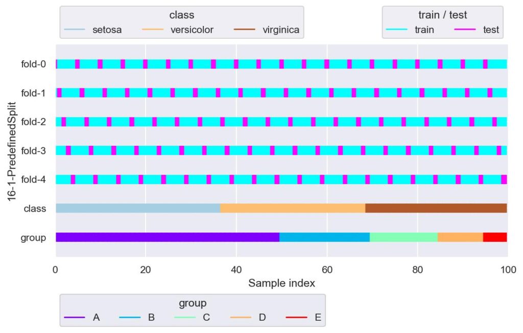

test_fold に自分で設定した配列を与えることで，自由度の高いデータ分割が行なえます．

ps = PredefinedSplit(test_fold=np.random.random_integers(low=0, high=1, size=10).tolist()*10)
plotter = FoldsPlotter(x=x, y=y, group=group, ylabel="16-2-PredefinedSplit")
for i, (train_idx, test_idx) in enumerate(ps.split()):
    plotter.add_plot(train_idx, test_idx)
plotter.show()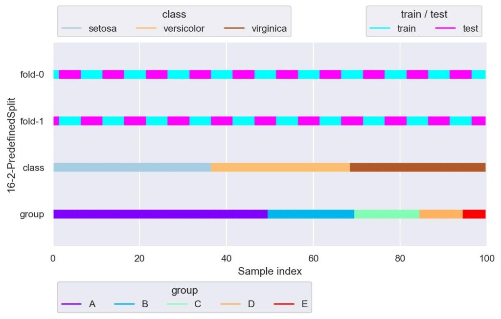

TimeSeriesSplit

sklearn.model_selection.TimeSeriesSplit(n_splits=5, *, max_train_size=None, test_size=None, gap=0)
・・・・時系列データを考慮したデータ分割手法で，検証用データを K 等分し，残りの検証用データよりも前のデータを学習用データとして用います．したがって，index=0 から始まるような検証用データにおける学習用データは取れないので，検証用データは K-1 個になります．引数 n_splits では，この K-1 を指定します．
  - n_splits: 検証用データを何等分するかを指定します．
  - max_train_size: 各 fold における学習用データの最大の個数を指定します．
  - test_size: 各 fold における検証用データの個数を指定します．
  - gap: 学習用データと検証用データを時間方向に離す個数を指定します．

実装例は以下です．

from sklearn.model_selection import TimeSeriesSplit

tss = TimeSeriesSplit(n_splits=2)
plotter = FoldsPlotter(x=x, y=y, group=group, ylabel="17-1-TimeSeriesSplit")
for i, (train_idx, test_idx) in enumerate(tss.split(X=x, y=y, groups=group)):
    plotter.add_plot(train_idx, test_idx)
plotter.show()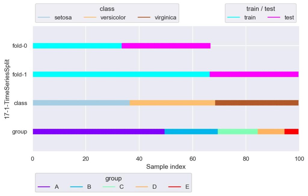

今回のデータは時系列データではありませんが，index の増加に伴い時間が経過するというふうに御覧ください．
データ分割で時系列を考慮しなければならない場合は，例えば未来のデータを求めるために未来のデータを用いることはありえないので，学習用データは検証用データよりも前の時間である必要があります．
そのため，他のデータ分割手法にはない引数が何種類かありますが，例えば n_splits=2 とだけ与えた場合は，上記のように，fold-1 の学習用データある時刻よりも前の時刻のすべてのデータが対象になります．

tss = TimeSeriesSplit(n_splits=5)
plotter = FoldsPlotter(x=x, y=y, group=group, ylabel="17-2-TimeSeriesSplit")
for i, (train_idx, test_idx) in enumerate(tss.split(X=x, y=y, groups=group)):
    plotter.add_plot(train_idx, test_idx)
plotter.show()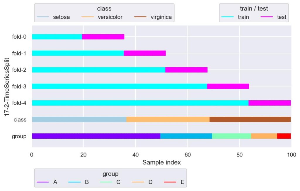

ある程度過去のデータを検証用データとして使いたい場合は，このように n_splits を大きくする必要があります．

tss = TimeSeriesSplit(n_splits=10, max_train_size=30, gap=5)
plotter = FoldsPlotter(x=x, y=y, group=group, ylabel="17-3-TimeSeriesSplit")
for i, (train_idx, test_idx) in enumerate(tss.split(X=x, y=y, groups=group)):
    plotter.add_plot(train_idx, test_idx)
plotter.show()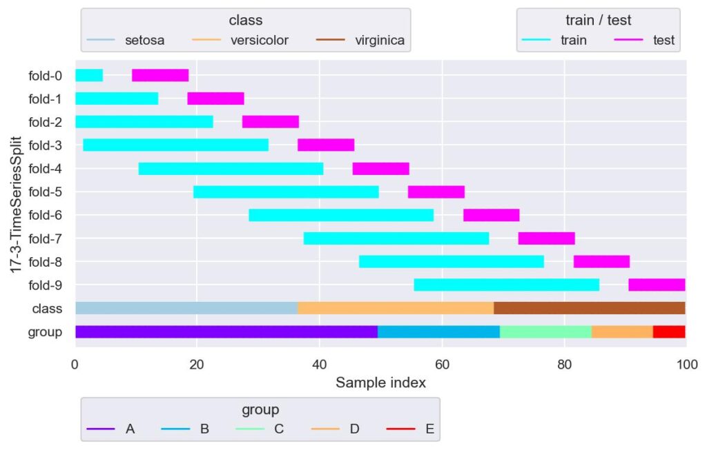

上図は n_splits の他に，max_train_size=30, gap=5 を引数として与えています．
上図の通り，学習用データがあって，gap 分開きがあって，その後検証用データがあるといった分割になります．
また，max_train_size=30 により，fold_3 以降の学習用データのデータ数は 30 に制限されています．
gap の使い所としては，本番実装を検討した際に，計算処理で遅延が発生し直近のデータの推論ができない場合などに用いることができそうです．
一方，max_train_size ですが，学習用データの長さを制限したいときに用いることができそうですが，学習用データの長さが可変にできないような機械学習を考えると，min_train_size も欲しいところです．
もし上記を実装したければ引数を逆算するか，あるいは，fold 数は減りますが，各 fold のループで学習用データが自分で設定した定数の min_train_size に満たない場合は continue することになるでしょう．